This article explores the Hessian matrix, a powerful mathematical tool for studying gradient descent. Before discussing the Hessian, we first need the basic concepts of gradients and the Jacobian matrix.
⭐ This article assumes familiarity with gradient descent and basic numerical analysis and linear algebra. Original article
Gradients and the Jacobian Matrix
Gradient descent requires derivative information at the current point of a function. For a function with multiple input directions, its gradient is the vector of partial derivatives in those directions.
The discussion above assumes a single output. When the function’s output is also a vector, we must take the gradient of each output element with respect to the inputs and stack them together. The resulting matrix is the Jacobian matrix.
For example:
- If a function $f$ takes three inputs $x1、x2、x3$ and produces one output $y$, its gradient is:
$$ \begin{equation} Grad = [\frac{\partial y}{\partial x_1}, \frac{\partial y}{\partial x_2}, \frac{\partial y}{\partial x_3}] \end{equation} $$
- If a function $f2$ takes three inputs $x1、x2、x3$ and produces three outputs $y1、y2、y3$, its Jacobian is:
$$ \begin{equation} Jacobian = \begin{bmatrix} \frac{\partial y_1}{\partial x_1} & \frac{\partial y_1}{\partial x_2}&\frac{\partial y_1}{\partial x_3} \ \frac{\partial y_2}{\partial x_1} & \frac{\partial y_2}{\partial x_2}&\frac{\partial y_2}{\partial x_3} \ \frac{\partial y_3}{\partial x_1} & \frac{\partial y_3}{\partial x_2}&\frac{\partial y_3}{\partial x_3} \end{bmatrix} \end{equation} $$
Second derivatives describe the curvature of a function in a particular direction $d$. This information helps anticipate the behavior of gradient descent. Along direction $d$:
-
If the second derivative is positive, the first derivative increases along $d$, and the function value decreases more slowly.
-
If the second derivative is negative, the first derivative decreases along $d$, and the function value decreases more quickly.
-
If the second derivative is zero, the first derivative remains constant along $d$, and the function value decreases at a constant rate.
⭐ Gradient descent reduces a loss function, so we analyze how derivatives change within a small local segment of a decreasing function. The decreasing side of a quadratic function is often used as an approximation, as in a second-order Taylor expansion or Newton’s method.
The Hessian Matrix
Like the Jacobian, the Hessian matrix contains information about the function’s second derivatives: $$ Hessian = \begin{bmatrix} \frac{\partial^2y}{\partial x_1\partial x_1} & \frac{\partial^2y}{\partial x_1\partial x_2}&\frac{\partial^2y}{\partial x_1\partial x_3} \ \frac{\partial^2y}{\partial x_2\partial x_1} & \frac{\partial^2y}{\partial x_2\partial x_2}&\frac{\partial^2y}{\partial x_2\partial x_3} \ \frac{\partial^2y}{\partial x_3\partial x_1} & \frac{\partial^2y}{\partial x_3\partial x_2}&\frac{\partial^2y}{\partial x_3\partial x_3} \end{bmatrix} $$ Because mixed second derivatives can be interchanged, namely $\frac{\partial^2y}{\partial x_1\partial x_2}=\frac{\partial^2y}{\partial x_2\partial x_1}$, the Hessian is a symmetric matrix. For a symmetric matrix, we can use eigendecomposition to study the relationship between eigenvalues and second derivatives and obtain a directional second derivative efficiently.
For a particular direction d, the second directional derivative can be written as $d^THd$. Therefore:
🔗 Second Directional Derivatives and Properties of the Hessian Matrix — CSDN
-
If d is an eigenvector of H corresponding to eigenvalue λ:
Since d is an eigenvector corresponding to λ, by definition: $$ Hd = \lambda d\ \Rightarrow d^THd=d^T\lambda d = \lambda d^Td=\lambda \ \ \ 对称矩阵d^T = d^- $$
The eigenvalue λ corresponding to that eigenvector is therefore the second derivative in that direction.
-
For another direction d, let $e_i$ be an eigenvector of $H$ with eigenvalue $\lambda_i$. From the result above, $$ \lambda_i=e_i^THe_i $$ Any direction $d=\sum_i^mt_ie_i$ is a linear combination of eigenvectors, where m is the number of eigenvalues and $t_i$ is the weight of the $i$th eigenvector. Thus: $$ d^THd=(\sum_i^mt_ie_i)^TH(\sum_i^mt_ie_i)=\sum_i^mt_ie_i^THt_ie_i=\sum_i^mt_i^2\lambda_i $$ The second derivative in an arbitrary direction that is not an eigenvector is therefore a weighted sum of all eigenvalues. In particular, this weighted sum describes an ellipsoid. With two eigenvalues, it is an ellipse, with the equation: $$ y=\frac{\lambda_1}{\frac{1}{t_1^2}}+\frac{\lambda_2}{\frac{1}{t_2^2}} $$
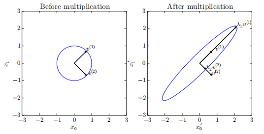
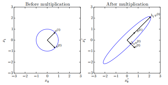
The figure shows that the maximum second derivative is determined by the largest eigenvalue, along the major semiaxis, and the minimum by the smallest eigenvalue, along the minor semiaxis.
Applications of the Hessian Matrix
With the definition of the Hessian established, we can use its properties to analyze optimization methods: identifying local maxima, local minima, and saddle points; choosing learning rates; and assessing how ill-conditioning affects gradient descent. We can also use the Hessian to implement Newton’s method as an optimization algorithm.
(End of section)